Michael Kalloniatis and Charles Luu
1. Introduction.
Visual acuity is the spatial resolving capacity of the visual system. This may be thought of as the ability of the eye to see fine detail. There are various ways to measure and specify visual acuity, depending on the type of acuity task used. Visual acuity is limited by diffraction, aberrations and photoreceptor density in the eye (Smith and Atchison, 1997). Apart from these limitations, a number of factors also affect visual acuity such as refractive error, illumination, contrast and the location of the retina being stimulated.
2. Types of acuity tasks.
Target detection requires only the perception of the presence or absence of an aspect of the stimuli, not the discrimination of target detail (figure 1).

The Landolt C and the Illiterate E are other forms of detection used in visual acuity measurement in the clinic. The task required here is to detect the location of the gap (figure 2).
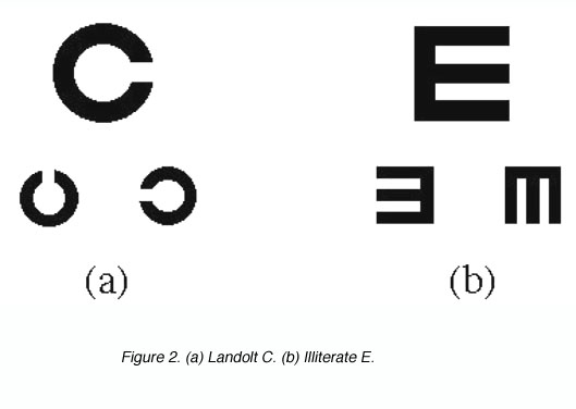
Figure 2. (a) Landolt C. (b) Illiterate E
Target recognition tasks, which are most commonly used in clinical visual acuity measurements, require the recognition or naming of a target, such as with Snellen letters. Test objects used here are large enough that detection is not a limiting factor (figure 3), but careful letter choice and chart design are required to ensure that letter recognition tasks are uniform for different letter sizes and chart working distances (Bailey and Lovie, 1976).

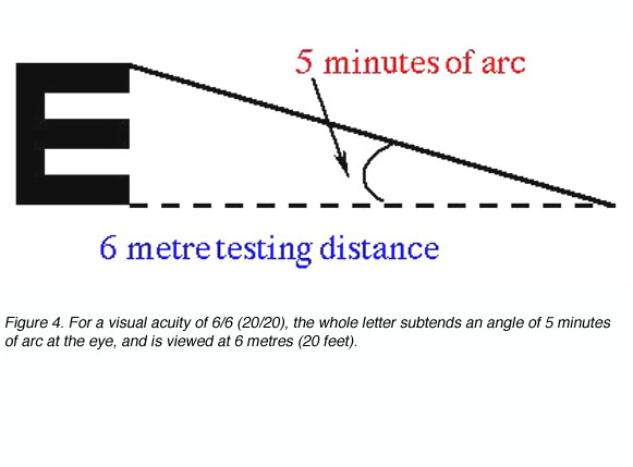
Snellen letters are constructed so that the size of the critical detail (stroke width and gap width) subtends 1/5th of the overall height. To specify a person’s visual acuity in terms of Snellen notation, a determination is made of the smallest line of letters of the chart that he/she can correctly identify. Visual acuity (VA) in Snellen notation is given by the relation:
VA = D’/D
where D’ is the standard viewing distance (usually 6 metres) and D is the distance at which each letter of this line subtends 5 minutes of arc (each stroke of the letter subtending 1 minute; figure 4).
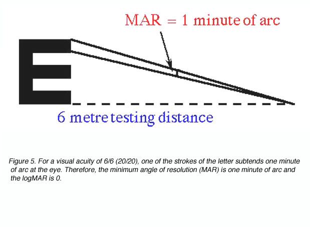
The reciprocal of the Snellen Notation equals the angle (in minutes of arc) which the strokes of the letter subtend at the person’s eye. This angle is also used to specify visual acuity (see Figure 5). It is called the minimum angle of resolution (MAR) and can also be given in log10 form, abbreviated as logMAR.
Some European countries specify their visual acuities in decimal form, which is simply the decimal of the Snellen fraction (Table 1).
| Snellen NotationMetric Imperial | MAR | logMAR | Decimal | |
| 6/60 | 20/200 | 10 | 1.0 | 0.10 |
| 6/48 | 20/160 | 8.0 | 0.9 | 0.13 |
| 6/38 | 20/125 | 6.3 | 0.8 | 0.16 |
| 6/30 | 20/100 | 5.0 | 0.7 | 0.20 |
| 6/24 | 20/80 | 4.0 | 0.6 | 0.25 |
| 6/19 | 20/60 | 3.2 | 0.5 | 0.32 |
| 6/15 | 20/50 | 2.5 | 0.4 | 0.40 |
| 6/12 | 20/40 | 2.0 | 0.3 | 0.50 |
| 6/9 | 20/30 | 1.6 | 0.2 | 0.63 |
| 6/7.5 | 20/25 | 1.25 | 0.1 | 0.80 |
| 6/6 | 20/20 | 1.00 | 0.0 | 1.00 |
| 6/4.8 | 20/16 | 0.80 | -0.1 | 1.25 |
| 6/3.8 | 20/12.5 | 0.63 | -0.2 | 1.58 |
| 6/3.0 | 20/10 | 0.50 | -0.3 | 2.00 |
Table 1. Relationship between Snellen notation, minimum angle of resolution and the logarithmic minimum angle of resolution.
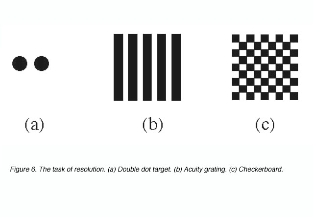
Target resolution thresholds are usually expressed as the smallest angular size at which subjects can discriminate the separation between critical elements of a stimulus pattern such as a pair of dots, a grating or a checkerboard (figure 6).

Figure 6. The task of resolution. (a) Double dot target. (b) Acuity grating. (c) Checkerboard
Target localisation involves discriminating differences in the spatial position of segments of a test object, such as a break or discontinuity in contour. Visual acuity measured in this way is called Vernier acuity (a type of hyperacuity) and the discontinuity is specified in terms of its angular size (figure 7).
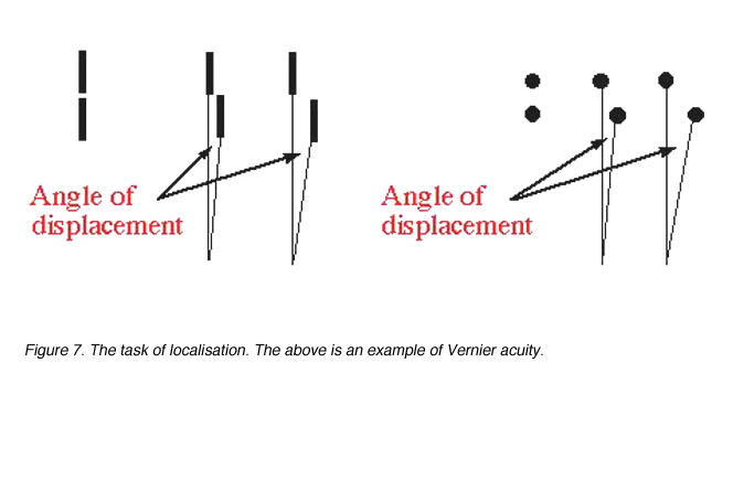
Figure 7. The task of localisation. The above is an example of Vernier acuity
Resolution, localisation or detection tasks produce hyperacuity or levels of performance over and above the recognition (normal visual acuity) limit and indicate that the mechanisms involved in making such judgements are not restricted to the retinal level (Westheimer, 1972; Waugh and Levi, 1995).
3. Visual acuity limitations.
For the smallest point to be detected or the finest detail to be resolved, requires a good optical system and appropriately spaced detectors. Visual acuity will be limited by one of these. Objects we look at will be imaged at the back of the eye. If we take a point source, the image will be distributed on the retina as a point spread function due to distortions created by the optics of the eye (figure 8).
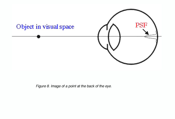
Figure 8. Image of a point at the back of the eye
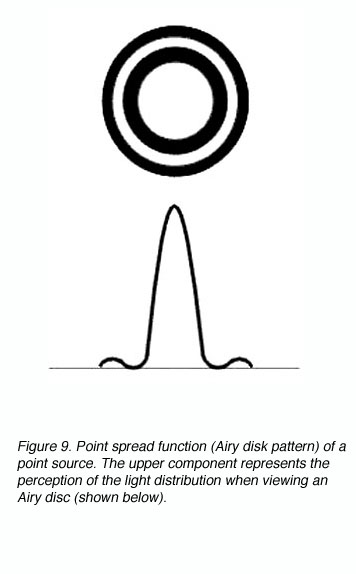
A point spread function describes the light distribution on the retina of a point source in visual space. An Airy disk pattern would be formed from a point source due to the diffraction of light (figure 9). A line spread function describes the light distribution of an extended source and is often used to simplify calculations.
The angular radius, a, of the first ring is given by:
a = 1.22 l/d
where l is the wavelength of light and d is the diameter of the pupil. The angular radius is in radians. To convert from radians to degrees, multiply by 180/p. Two point sources produce two point spread functions at the back of the eye (figure 10). These two points are said to be just resolved if they meet Rayleigh’s criterion (see below). Clearly, if the retinal image of the two point sources was not degraded, it would be possible to have higher resolution limits (with the appropriate detector array).
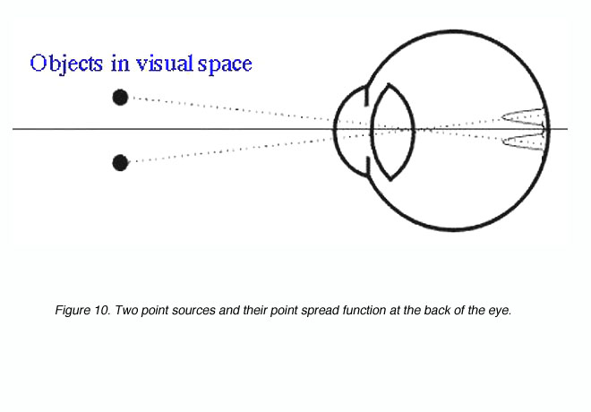
Figure 10. Two point sources and their point spread function at the back of the eye
4. Raleigh’s criteria.
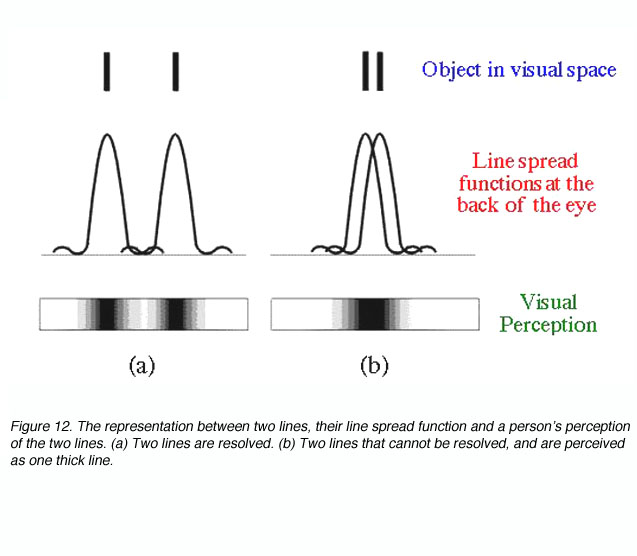
Raleigh’s criterion is used to calculate the resolution of the eye for stimuli that are degraded by the optics of the eye. The criterion states that two points or lines are just resolved if the peak of the point spread function lies on the first trough of the other point spread function (figure 11).
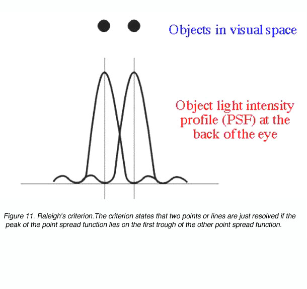
Figure 11. Raleigh’s criterion
Two point are resolved if their angular separation, as
is:
as = 1.22l/d
In effect this equation mathematically states that resolution is possible if two objects are separated by the width of their point spread function. If two objects are within this distance, (figure 12), our perception of them is that of one uniform distribution (part b) and hence we will not be able to discern the two objects.
5. Dimension of the retinal mosaic.
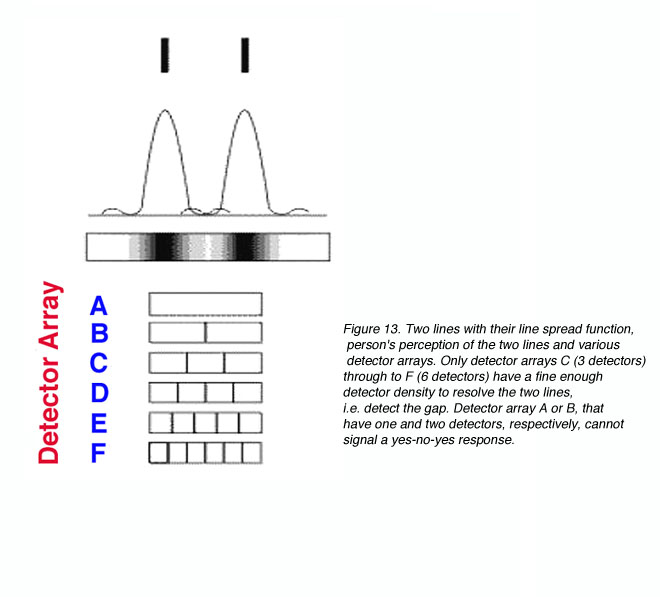
Other than diffraction limiting visual acuity according the Raleigh’s criterion, retinal cone spacing is another limiting factor, at least within the central two degrees (Green, 1970). Helmholtz proposed that a grating would be resolved if there is a row of unstimulated cone in between rows of stimulated cones. This is considered the Yes-No-Yes response of the cone receptors. For example, if two lines are to be resolved, a detector array needs to be fine enough to detect a gap in between the two lines (figure 13). From figure 13, it can be seen that detectors A and B will not be able to resolve the two lines. However, with a fine detector array of detectors C, D, E and F, the two lines would be resolved.
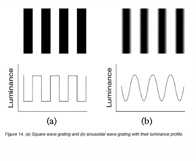
The same principle applies to sinusoidal gratings where a detector array must be fine enough to detect the gap between the lines or gratings. The bars of a sinusoidal grating do not change abruptly as with square wave gratings (figure 14).

Figure 14. (a) Square wave grating and (b) sinusoidal wave grating with their luminance profile
Gratings can be used as another method of measuring visual acuity. Visual acuity in Snellen notation can be expressed in spatial frequency and vice versa (figure 15).

Figure 15. Visual acuity in Snellen notation and its conversion to spatial frequency
Sinusoidal gratings were used by Campbell and Green (1965) to determine the maximum resolution of the eye. They used interference patterns generated by a laser to bypass the optics of the eye to create a sinusoidal grating at the back of the eye. They found that the maximum resolution was about 60 cycles per degree, whereas a free viewing screen resulted in reduced resolution capabilities. More recent work on photoreceptor density and spatial resolution has shown that the receptor array in the human visual system can resolve in the order of 6/1 (20/3) or ~150 cycles/degree (Curcio et al, 1990; Miller et al., 1996; Roorda and Williams, 1999). Cone spacing at the fovea is approximately 2.5 um (Curcio et al, 1990) or approximately 28 seconds of arc. Based on cone spacing, a maximum of about 60 cycles per degree is possible, which is well above conventional clinical measures as this does not compensate for the optics of the eye and post-receptoral neural processing.
6. Factors affecting visual acuities.
Apart from the two main limiting factors above, visual acuity also depends on a number of factors including:
- Refractive error
- Size of the pupil
- Illumination
- Time of exposure of the target
- Area of the retina stimulated
- State of adaptation of the eye
- Eye movement
1. Refractive error.
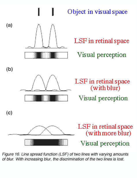
Refractive errors will affect visual acuity by causing defocus at the retina. Defocus will blur out fine detail, sharp edges and contrast sensitivity by affecting its point spread function (figure 16).
Refractive errors such as myopia (short-sightedness) and hyperopia (long-sightedness) causes the point spread function to spread more laterally. Therefore, affecting resolution (figure 17). The image at the back of the eye of an object is focussed sharply on the retina in an emmetropic eye. In a myopic eye, the optical system can be considered to be too strong, thus the image is focussed in front of the retina. The reverse occurs with a hyperopic eye where the optical system is too weak so the image is focussed behind the retina.

Figure 17. Point spread function at the back of the eye with different refractive errors
2. Pupil size.
The size of the pupil is an important factor affecting visual acuity. Large pupils allows more light to stimulate the retina and reduces diffraction but resolution will be affected by aberrations of the eye. On the other hand, a small pupil will reduce optical aberrations but resolution will be diffraction limited. Therefore, a mid-size pupil of about 3 mm to 5 mm would be optimal, as this is a compromise between the diffraction and aberration limits (Atchison et al, 1979; Smith and Atchison, 1997). As noted earlier, pupil area affects the size of the point spread function, and hence resolution.
3. Illumination.
For recognition tasks, visual acuity is greatly affected by the level of background luminance (figure 18). Two branches are evident, the lower belongs to the rod (scotopic) function and the upper to the cone (photopic) function. Note the asymptote for both indicating the maximum visual acuity (arrows). The cone branch has a long “linear” range of about 3 log units which asymptote at the photopic level of about 300 cd/m2.

One theory put forward by Hecht is that within the rod population and within the cone population, there are differing sensitivities which are distributed randomly. Therefore, at high luminance, all cells are active for a high level of visual acuity. At low luminances, only cells sensitive to that level of luminances are active and because they are distributed randomly, the retinal mosaic is coarser thus a lower level of visual acuity is achieved (Graham, 1965).
Another possible explanation is that under limited quantal availability, quantal capture is more probable in the para-central and peripheral retinal due to greater spatial summation. Since photoreceptors density in this area is low, resolution is poorer. As light levels increase, quantal capture occurs more successfully at the central retinal (macula and fovea). A higher level of visual acuity is achieved due to the high photoreceptor density.
4. Time of exposure of the target.
To detect a small bright spot, detection is greatly dependent on the quantity of light rather than the exposure time. However, to detect a line, the acuity, (reciprocal width of the line) is proportional to the exposure time. There is no simple acuity-exposure time relationship for the resolution of the target.
5. Area of the retina stimulated.
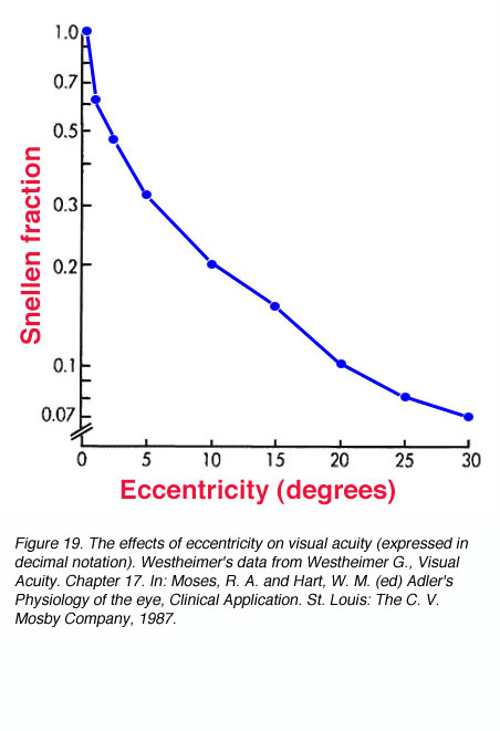
Due to the densely packed cones at the fovea, visual acuity is the greatest at the centre of fixation. At a distance of 5 minutes of arc from the centre of fixation, there is a measurable loss in visual acuity. At 10 minutes of arc (1/6 of a degree) from fixation, there is a 25 % loss of visual acuity (figure 19). When comparisons were made of cone packing density and photopic resolution, close correlation was evident up to approximately two degrees eccentricity (Green, 1970). At larger eccentricities, visual acuity is worse than that predicted by cone spacing that may indicate that other post-receptoral retinal element is the limiting factor (see discussion below for scotopic visual acuity).
6. State of adaptation of the eye.
Highest level of visual acuity is achieved if the eye is adapted to the same level as the test luminance for test luminances of 34 cd/m2 to 34,000 cd/m2. For test luminances less than 34cd/m2, adapting to a lower luminance will achieve a slightly better acuity.
The high density of cones at the fovea is responsible for the high levels of visual acuity under photopic conditions. Under scotopic conditions, the AII amacrine cell which is an interneuron identified in the primate retina (Kolb, et al, 1992; Wassle et al, 1995) appears to limit resolution. Maximum scotopic acuity occurs at ~5-15o eccentricity, which corresponding to the AII amacrine cell density, while peak rod density occurs at about 15-20o. The arrow in figure 20 shows that at eccentricities less than 15o, scotopic acuity is limited by the AII amacrine cell. Beyond 15o, scotopic acuity is limited by the midget ganglion cell (P cell; Mills and Massey, 1999).

As noted above, a similar process may occur in the photopic system (Green, 1970), where photopic resolution beyond an eccentricity of two degrees, falls below that predicted by cone density. The works by both Green (1970) and Mills and Massey (1999) provide evidence that post-receptoral processing is another factor that may limit visual acuity.
Eye movement.
During steady fixation, the eyes are in constant motion. Under these conditions, retinal images traverse a distance of about 3 minutes of arc in one second.
Contrast Sensitivity
Contrast is an important parameter in assessing vision. Visual acuity measurement in the clinic use high contrast, that is, black letters on a white background. In reality, objects and their surroundings are of varying contrast. Therefore, the relationship between visual acuity and contrast allows a more detailed understanding of our visual perception.
Grating patterns are used as a means of measuring the resolving power of the eye because the gratings can be adjusted to any size. The contrast of the grating is the differential intensity threshold of a grating, which is defined as the ratio:
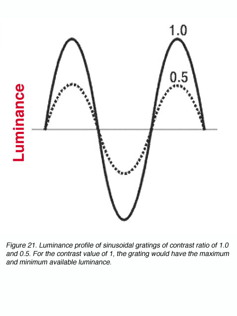
C = (Lmax – Lmin) / (Lmax + Lmin)
where C can have a value between 0.0 and 1.0; sometimes C is called the modulation, Raleigh or Michelson contrast (figure 21). The luminance of contrast gratings vary in a sinusoidal manner (figure 21). This allows the contrast of the grating to be altered without changing the average luminance of the screen displaying the gratings.
The size of the bars of the grating can be expressed in terms of the number of cycles (one cycle consists of one light bar plus one dark bar of the grating) per degree subtended at the eye. This is called the spatial frequency of the grating and can be thought of as a measure of the fineness or coarseness of the grating. The units can be cycles per degree (figure 22).

We can determine the sensitivity of the visual system as a function of grating size (spatial frequency). The contrast of the grating patterns is adjusted to determine the threshold for a given spatial frequency. That is, with a given spatial frequency, the contrast can be lowered until detection of the grating becomes impossible (contrast threshold). The reciprocal of this contrast threshold is called contrast sensitivity.
The contrast required for the visual system to reach a certain threshold can be expressed as a sensitivity on a decibel (dB) scale (contrast sensitivity in dB = -20 log10C). A plot of (contrast) sensitivity versus spatial frequency is called the spatial contrast sensitivity function (SCSF, or usually abbreviated to CSF).
Contrast Sensitivity Function (CSF)
Under photopic conditions, contrast sensitivity measurements reveal a band-pass function when using sinusoidal gratings (figure 23). The peak of the CSF function is in the mid-spatial range and only under high contrast conditions, is resolution at its maximal level.
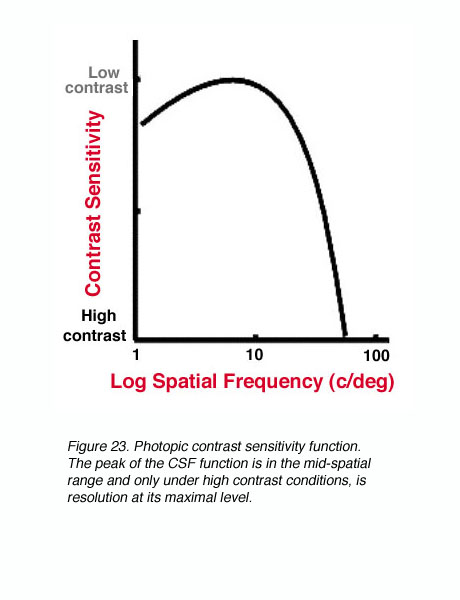
Figure 23. Photopic contrast sensitivity function
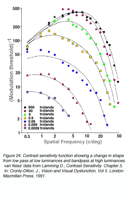
The shape and critical parameters of the CSF depends on a number of factors including: the mean luminance of the grating, whether the luminance profiles of the gratings are sinusoidal or square waveforms, the level of defocus, and the clarity of the optics of the eye. At low light levels, maximum contrast sensitivity is approximately 8% and maximum resolution is approximately 6 cycles per degree. As mean light levels increase, the peak of the contrast sensitivity function is now close to 0.5% contrast and the high spatial frequency cut off is at about 50 to 60 cycles per degree (~6/3 or 20/10). Also shown in figure 24, at photopic light levels, the peak contrast sensitivity is at approximately 5 to 10 cycles per degree (van Ness and Bouman, 1967).
The contrast sensitivity function provides a more thorough representation of the visual system. For example, the pivotal visual developmental study of Harwerth et al. (1986) characterized the changes in the contrast sensitivity function after different periods of monocular deprivation in monkeys. The loss of sensitivity in the mid to high spatial frequencies was profound during abnormal visual development, with increased deprivation leading to further contrast losses. Not only will certain disease/disorders of the eye reduce visual acuity, contrast sensitivity will also be affected (Arden, 1978). For example, patients with multiple sclerosis will have mid to low contrast sensitivity losses (figure 25 – B), while patients with cataracts will have an overall reduction in contrast sensitivity (figure 25 – C). Mild refractive error or mild amblyopia, will lead to a CSF similar to D in figure 25, with more severe refractive errors or severe amblyopia, resulting in a CSF similar to curve C.
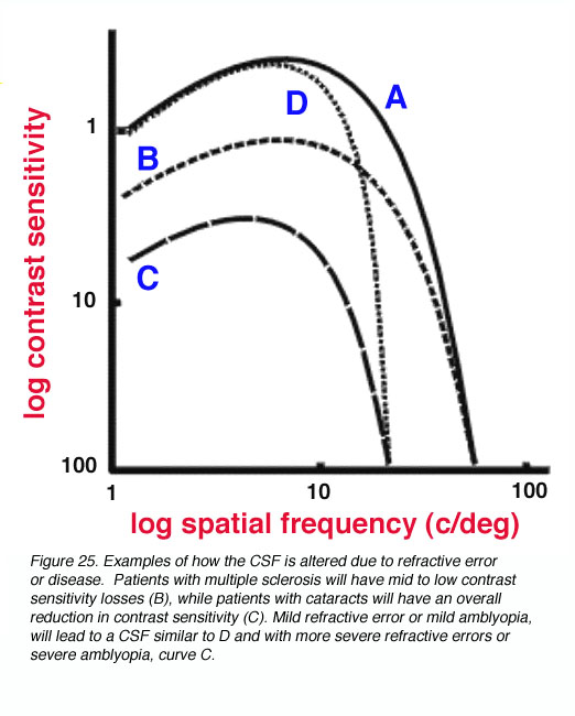
Figure 25. Examples of how the CSF is altered due to refractive error or disease
8. Spatial Summation.
Spatial summation describes the eye’s ability to summate or add up quanta over a certain area. This area over which spatial summation operates is called the critical diameter. According to Ricco’s Law, within this critical diameter, threshold is reached when the total luminous energy reaching a constant value (k). Threshold is reached when the product of luminance (L) and stimulus area (A) equals or exceeds this constant value. In another words, when luminance is halved, a doubling in stimulus area is required to reach threshold. When luminance is doubled, the stimulus area can be halved and still reach threshold. Ricco’s Law is expressed as:
L. An = k
where L is the luminance of the stimulus, A is the area of the stimulus, k is a constant value and n describes whether spatial summation is complete (n=1) or partial (0<n<1). No spatial summation occurs when n = 0. Critical area varies with eccentricity. Ricco’s Law holds for an area of 30 minutes of arc in the parafoveal area (4 to 7o eccentricity) and increasing to an area of about 2o at an eccentricity of 35o (Davson, 1990).
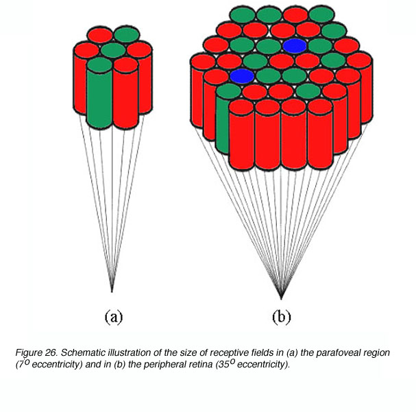
Spatial summation occurs due to the convergence of photoreceptors onto ganglion cells. This convergence of photoreceptors form a receptive field thus stimulating different photoreceptor within this receptive field would result in one signal. Receptive field sizes vary with eccentricity (figure 26), and helps explain the reason why critical area varies with eccentricity (Shapley and Enroth-Cugell, 1984). Clearly, the size of spatial summation (functional receptive field), will limit resolution capabilities as outlined earlier.
A schematic spatial summation graph is shown in figure 27. A simple logarithmic transform of L.A=k results in the logL versus logA plot having a straight line with a slope of -1 (complete spatial summation within Ricco’s law). Outside the critical area, such a plot has a slope of 0, indicating that the size of the target does not affect threshold.
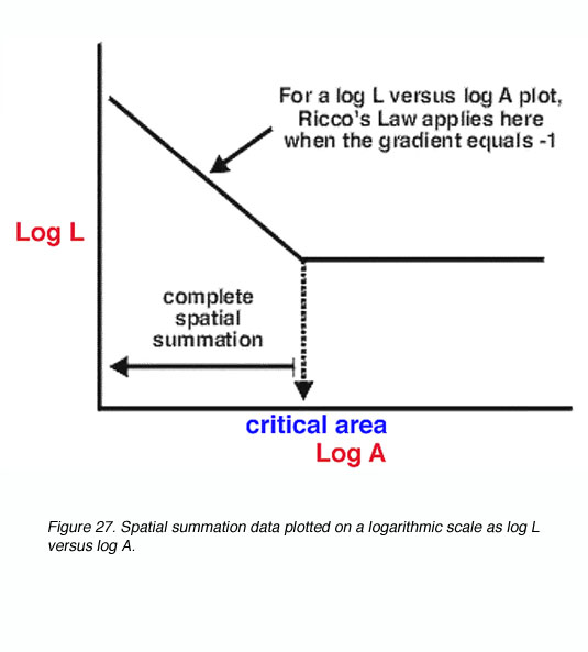
Figure 27. Spatial summation data plotted on a logarithmic scale as log L versus log A
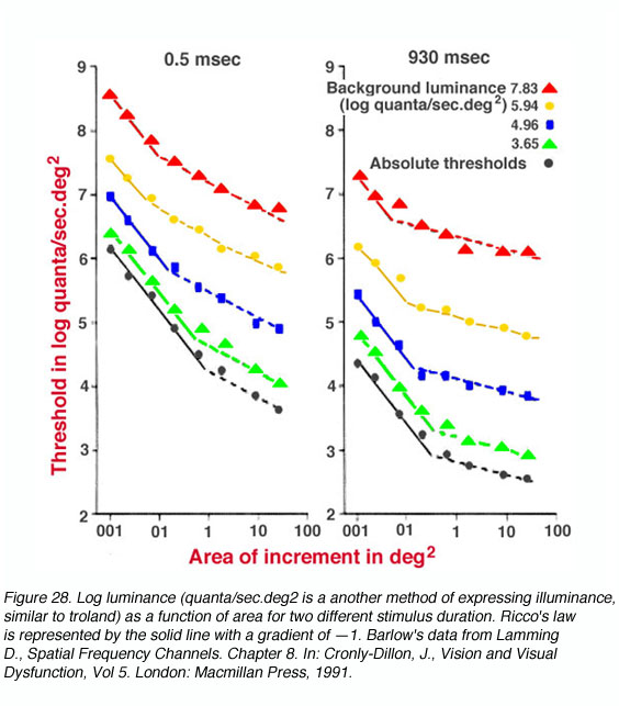
Figure 28 shows data on spatial summation where spots of light with different background luminance are presented 6.5o nasally from the fovea. Ricco’s law of complete spatial summation holds when the gradient is —1 (solid line). Note that the critical area is larger for low luminance and smaller for high luminance. Such a change reflects the functional alteration of receptive field size with changes in adaptation level (Shapley and Enroth-Cugell, 1984).
References.
Arden GB. The importance of measuring contrast sensitivity in cases of visual disturbance. Br J Ophthalmol. 1978;62:198–209. [PubMed] [Free Full text in PMC]
Atchison DA, Smith G, Efron N. The effect of pupil size on visual acuity in uncorrected and corrected myopia. Am J Optom Physiol Opt. 1979;56:315–323.[PubMed]
Bailey IL, Lovie JE. New design principles for visual acuity letter charts. Am J Optom Physiol Opt. 1976;53:740–745. [PubMed]
Campbell FW, Green DG. Optical and retinal factors affecting visual resolution. J Physiol. 1965;181:576–593. [PubMed]
Cronly-Dillon, J. (1991) Vision and Visual Dysfunction, Vol 5. London: Macmillan Press.
Curcio CA, Sloan KR, Kalina RE, Hendrickson AE. Human photoreceptor topography. J Comp Neurol. 1990;292:497–523. [PubMed]
Davson H. . Davson’s physiology of the eye. 5th ed. London: Macmillan Academic and Professional Ltd. 1990
Graham CH. . Vision and visual perception. New York: John Wiley and Sons, Inc. 1965
Green DG. Regional varitations in the visual acuity for interference fringes on the retina. J Physiol. 1970;207:351–356. [PubMed] [Free Full text in PMC]
Harwerth RS, Smith EL, Duncan GC, Crawford ML, von Noorden GK. Multiple sensitive periods in the development of the primate visual system. Science.1986;232:235–238. [PubMed]
Hecht S. The relation between visual acuity and illumination. J Gen Physiol. 1928;11:255–281. [PubMed]
Helmholtz HV. (). Handbuch der physiologischen optik. Leipzig: Leopold Voss. 1867
Kolb H, Linberg KA, Fisher SK. Neurons of the human retina: a Golgi study. J Comp Neurol. 1992;318:147–187. [PubMed]
Lamming D. Contrast sensitivity. In: Cronly-Dillon J, editor. Vision and visual dysfunction. Vol. 5. London: Macmillan Press; 1991.
Lamming D. Spatial frequency channels. In: Cronly-Dillon J, editor. Vision and visual dysfunction. Vol. 5. London: Macmillan Press; 1991.
Mills SL, Massey SC. AII amacrine cells limit scotopic acuity in central macaque retina: a confocal analysis of calretinin labeling. J Comp Neurol. 1999;411:19–34.[PubMed]
Riggs LA. Visual acuity. In: Graham CH, editor. Vision and visual perception. New York: John Wiley and Sons, Inc.; 1965.
Roorda A, Williams DR. The arrangement of the three cone classes in the living human eye. Nature. 1999;397:520–522. [PubMed]
Shapley R, Enroth-Cugell C. Visual adaptation and retinal gain controls. Prog Retinal Res. 1984;3:263–346.
Smith G, Atchison DA. The eye and visual optical instrument. New York: Cambridge University Press. 1997
van Nes FL, Bouman MA, Maarten A. Spatial modulation transfer in the human eye. J Opt Soc Am. 1967;57:401–406.
Wässle H, Grunert U, Chun MH, Boycott BB. The rod pathway of the macaque monkey retina: identification of AII-amacrine cells with antibodies against calretinin.J Comp Neurol. 1995;361:537–551. [PubMed]
Waugh SJ, Levi DM. Spatial alignment across gaps: contributions of orientation and spatial scale. J Opt Soc Am A Opt Image Sci Vis. 1995;12:2305–2317.[PubMed]
Westheimer G. Visual acuity and spatial modulation thresholds. In: Jameson D, Hurvich LM, editor. Handbook of sensory physiology. Visual psychophysics. Vol. 7. Berlin: Springer-Verlag; 1972. pt. 4. p. 170-187.
Westheimer G. Visual acuity. In: Moses RA, Hart WM, editor. Adler’s physiology of the eye. Clinical application. St. Louis (MO): The C.V. Mosby Company; 1987.
Last Update: June 5, 2007.
The author

Michael Kalloniatis was born in Athens Greece in 1958. He received his optometry degree and Master’s degree from the University of Melbourne. His PhD was awarded from the University of Houston, College of Optometry, for studies investigating colour vision processing in the monkey visual system. Post-doctoral training continued at the University of Texas in Houston with Dr Robert Marc. It was during this period that he developed a keen interest in retinal neurochemistry, but he also maintains an active research laboratory in visual psychophysics focussing on colour vision and visual adaptation. He was a faculty member of the Department of Optometry and Vision Sciences at the University of Melbourne until his recent move to New Zealand. Dr. Kalloniatis is now the Robert G. Leitl Professor of Optometry, Department of Optometry and Vision Science, University of Auckland. e-mail: m.kalloniatis@unsw.edu.au
The author

Charles Luu was born in Can Tho, Vietnam in 1974. He was educated in Melbourne and received his optometry degree from the University of Melbourne in 1996 and proceeded to undertake a clinical residency within the Victorian College of Optometry. During this period, he completed post-graduate training and was awarded the post-graduate diploma in clinical optometry. His areas of expertise include low vision and contact lenses. During his tenure as a staff optometrist, he undertook teaching of optometry students as well as putting together the “Cyclopean Eye”, in collaboration with Dr Michael Kalloniatis. The Cyclopean Eye is a Web based interactive unit used in undergraduate teaching of vision science to optometry students. He is currently in private optometric practice as well as a visiting clinician within the Department of Optometry and Vision Science, University of Melbourne.